R中网络分析常用的包igraph（包含算法与可视化）、tidygraph（使用tidy封装了igraph算法）、 vizNetwork (网络可视化htmlwidgets，使用viz.js)、ggraph（ggplot2 可视化网络）、statnet（用于网络数据表示、可视化、分析和模拟的集成工具）、RCy3（使用 CyREST 在R和 Cytoscape之间进行通信，允许使用 Cytoscape 点击式可视界面查看、探索和操作任何图形）。

igraph

library(igraph,warn.conflicts = FALSE)
library(igraphdata)


data(macaque)
class(macaque)
## [1] "igraph"
macaque
## IGRAPH f7130f3 DN-- 45 463 -- 
## + attr: Citation (g/c), Author (g/c), shape (v/c), name (v/c)
## + edges from f7130f3 (vertex names):
##  [1] V1 ->V2     V1 ->V3     V1 ->V3A    V1 ->V4     V1 ->V4t    V1 ->MT    
##  [7] V1 ->PO     V1 ->PIP    V2 ->V1     V2 ->V3     V2 ->V3A    V2 ->V4    
## [13] V2 ->V4t    V2 ->VOT    V2 ->VP     V2 ->MT     V2 ->MSTd/p V2 ->MSTl  
## [19] V2 ->PO     V2 ->PIP    V2 ->VIP    V2 ->FST    V2 ->FEF    V3 ->V1    
## [25] V3 ->V2     V3 ->V3A    V3 ->V4     V3 ->V4t    V3 ->MT     V3 ->MSTd/p
## [31] V3 ->PO     V3 ->LIP    V3 ->PIP    V3 ->VIP    V3 ->FST    V3 ->TF    
## [37] V3 ->FEF    V3A->V1     V3A->V2     V3A->V3     V3A->V4     V3A->VP    
## [43] V3A->MT     V3A->MSTd/p V3A->MSTl   V3A->PO     V3A->LIP    V3A->DP    
## + ... omitted several edges
data(Koenigsberg)
Koenigsberg
## IGRAPH 227bd5e UN-- 4 7 -- The seven bidges of Koenigsberg
## + attr: name (g/c), name (v/c), Euler_letter (v/c), Euler_letter (e/c),
## | name (e/c)
## + edges from 227bd5e (vertex names):
## [1] Altstadt-Loebenicht--Kneiphof          
## [2] Altstadt-Loebenicht--Kneiphof          
## [3] Altstadt-Loebenicht--Lomse             
## [4] Kneiphof           --Lomse             
## [5] Vorstadt-Haberberg --Lomse             
## [6] Kneiphof           --Vorstadt-Haberberg
## [7] Kneiphof           --Vorstadt-Haberberg

第一行中，字符编码的意义：

D或者U代表有向（undireted）或者无向（undireted）
N：第二个字母是“N”，用于命名图形。如果是破折号表示图表没有命名。
W: 第三个字母是“W”，如果图形是加权的(换句话说，如果图形是值图，第2.4节)。非加权图在这个位置是破折号。
B：第四个字母是“B”，代表是双向的（two-mode）; For unipartite (one-mode) graphs a dash is printed here。

旁边两个数字代表顶点vertices,nodes数和边edge,links数。

neighbors(graph, v, mode = c("out", "in", "all", "total"))返回顶点被edges连接的邻接顶点，对于无向graph而言，mode参数没有意义，对于有向图，mode为“out”时，连接为outgoing【外连接】,即顶点为边的尾部。

macaque %>% ends('V1|V2') #获取边的两端
##      [,1] [,2]
## [1,] "V1" "V2"
macaque %>% tail_of('V1|V2') #获取有向图边的尾部节点
## + 1/45 vertex, named, from f7130f3:
## [1] V1
macaque %>% head_of('V1|V2') #头部
## + 1/45 vertex, named, from f7130f3:
## [1] V2
macaque %>% neighbors('PIP', mode = "out")
## + 8/45 vertices, named, from f7130f3:
## [1] V1 V3 V4 VP MT PO DP 7a
E(macaque)[from("PIP")]
## + 8/463 edges from f7130f3 (vertex names):
## [1] PIP->V1 PIP->V3 PIP->V4 PIP->VP PIP->MT PIP->PO PIP->DP PIP->7a
E(macaque)[c('V1|V2', 'V2|V3A', 'V3A|V4')]
## + 3/463 edges from f7130f3 (vertex names):
## [1] V1 ->V2  V2 ->V3A V3A->V4

子图与组件（components）

induced_subgraph可以根据给出的顶点生成子图。

V(macaque)['V1', 'V2', nei('V1'), nei('V2')] %>%
  induced_subgraph(graph = macaque)
## IGRAPH 145ddad DN-- 16 156 -- 
## + attr: Citation (g/c), Author (g/c), shape (v/c), name (v/c)
## + edges from 145ddad (vertex names):
##  [1] V1 ->V2     V1 ->V3     V1 ->V3A    V1 ->V4     V1 ->V4t    V1 ->MT    
##  [7] V1 ->PO     V1 ->PIP    V2 ->V1     V2 ->V3     V2 ->V3A    V2 ->V4    
## [13] V2 ->V4t    V2 ->VOT    V2 ->VP     V2 ->MT     V2 ->MSTd/p V2 ->MSTl  
## [19] V2 ->PO     V2 ->PIP    V2 ->VIP    V2 ->FST    V2 ->FEF    V3 ->V1    
## [25] V3 ->V2     V3 ->V3A    V3 ->V4     V3 ->V4t    V3 ->MT     V3 ->MSTd/p
## [31] V3 ->PO     V3 ->PIP    V3 ->VIP    V3 ->FST    V3 ->FEF    V3A->V1    
## [37] V3A->V2     V3A->V3     V3A->V4     V3A->VP     V3A->MT     V3A->MSTd/p
## [43] V3A->MSTl   V3A->PO     V3A->FST    V3A->FEF    V4 ->V1     V4 ->V2    
## + ... omitted several edges

在图论中，连通图基于连通的概念。在一个无向图 G 中，若从V_i到V_j有路径相连（当然从v_j到V_i也一定有路径），则称i和j是连通的。如果 G 是有向图，那么连接i和j的路径中所有的边都必须同向。如果图中任意两点都是连通的，那么图被称作连通图。

通过is_connected(graph,mode = c("weak","strong)) 判断，对于无向图，mode参数被忽略。

强连通图（Strongly Connected Graph）是指在有向图G中，如果对于每一对vi、vj，vi≠vj，从vi到vj和从vj到vi都存在路径，则称G是强连通图。

弱连通图：将有向图的所有的有向边替换为无向边，所得到的图称为原图的基图。如果一个有向图的基图是连通图，则有向图是弱连通图。

is_connected(macaque, mode = "strong")
## [1] TRUE
is_connected(macaque, mode = "weak")
## [1] TRUE

连通分量（connected components）

igraph使用clusters或者components获取连通分量，两个函数是相同的。

g <- sample_gnp(20, 1/20)
(clu <- components(g))
## $membership
##  [1] 1 2 1 1 2 2 3 1 4 1 1 5 1 6 7 2 1 1 2 5
## 
## $csize
## [1] 9 5 1 1 2 1 1
## 
## $no
## [1] 7
plot(g)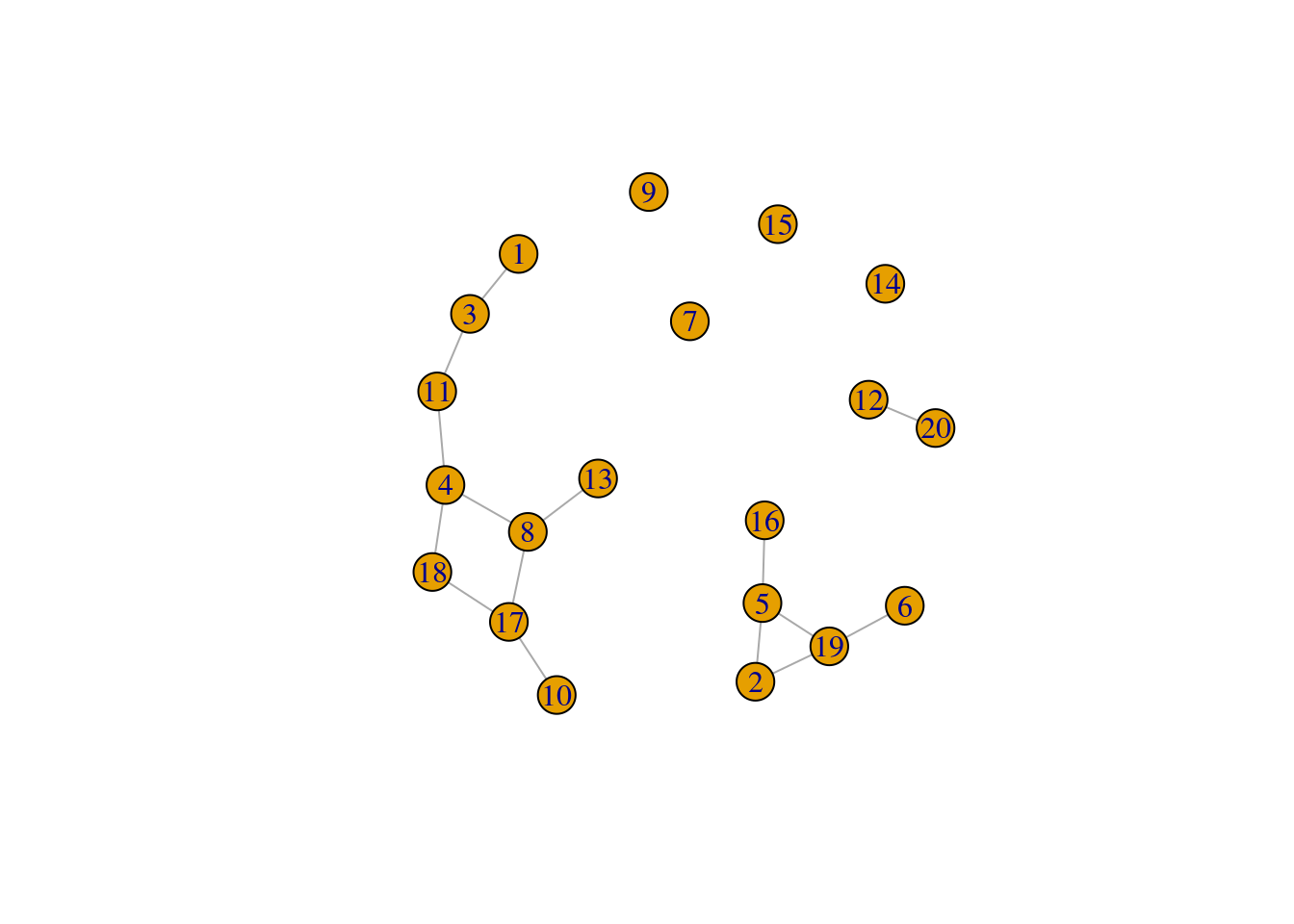

groups(clu)
## $`1`
## [1]  1  3  4  8 10 11 13 17 18
## 
## $`2`
## [1]  2  5  6 16 19
## 
## $`3`
## [1] 7
## 
## $`4`
## [1] 9
## 
## $`5`
## [1] 12 20
## 
## $`6`
## [1] 14
## 
## $`7`
## [1] 15

顶点与边可以使用索引操作：

V(macaque)[1:4]
## + 4/45 vertices, named, from f7130f3:
## [1] V1  V2  V3  V3A
V(macaque)[c('V1', 'V2', 'V3', 'V3A')]
## + 4/45 vertices, named, from f7130f3:
## [1] V1  V2  V3  V3A

R网络分析note

Liripo

2021-11-04

igraph

子图与组件（components）